

PART 3 – Signal Processing
In Section 2 we studied the 'OSCIL' unit generator. This was created in an orchestra file. We then made several different score files to use this orchestra to do additive synthesis, create beat frequencies and complex frequencies.
We shall now turn our attention to some common signal processing techniques:
- A – Amplitude Envelopes – the 'ADSR' shapes found on synthesisers
- B – Chorusing – a means of enriching a sound
- C – Frequency Modulation – the basis of the Yamaha synthesis technique (FM)
- D – Ring Modulation – multiplying two oscillators to distort the harmonic ratios
- E – Buzz – generating partials using a 'complex oscil' unit generator
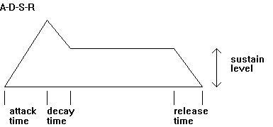
We are probably familiar with the enveloping functions on many synthesisers: Attack-Decay-Sustain-Release (ADSR):
The following diagram summarises this:
The Csound signal processing unit LINEN models this process in software. This is a three-part time-based amplitude envelope, in which the:
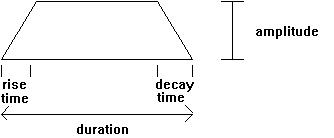
The following diagram illustrates the data flow of the LINEN generator:
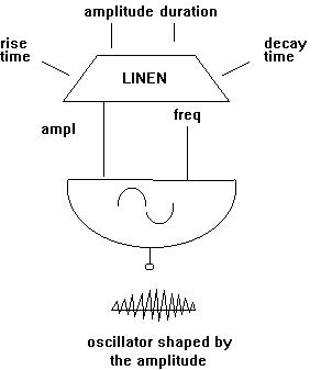
The following is an orchestra which uses LINEN:
;toot3.orc
sr     =  22050
kr     =   1470
ksmps  =     15
nchnls =      1
instr 3

;output generator ampl rise dur decay
k1      linen     p4,  p6,  p3, p7
a1      oscil     k1,  p5,  1
out    a1
endin
The following is a score to provide some notes and other data for this orchestra:
;toot3.sc

f1  0  4096  10  1	;sine wave made with GEN10

;p1    p2    p3   p4     p5      p6     p7
;instr start dur  ampl   freq    rise   decay
i3     0     1    10000  440     .5     .7
i3     1.5   1    10000  440     .9     .1
i3     3     1    5000   880     .02    .99
i3     4.5   1    5000   880     .7     .01
i3     6     2    20000  220     .5     .5
e
OK – this gives us the general idea, but too many different parameters are changing at once. Try the following score, which keeps all the parameters the same except 'rise' (which gets shorter) for the first 7 notes, then holds that steady while 'decay' starts to get longer for the next 7 notes. The procedure here is important. It's 'scientific method' procedure, where one tries to keep all the variables the same except one, so that one can clearly observe what happens when that one variable alters.
;toot3.sc - alternative version no.1

f1  0  4096  10  1

;p1    p2    p3   p4     p5    p6   p7
;instr start dur  ampl   freq  rise decay
i3     0     1.5  10000  440   .9   .7
i3     2     1.5  10000  440   .7   .7
i3     4     1.5  10000  440   .5   .7
i3     6     1.5  10000  440   .3   .7
i3     8     1.5  10000  440   .15  .7
i3     10    1.5  10000  440   .04  .7
i3     12    1.5  10000  440   .02  .7
i3     14    1.5  10000  440   .02  .02
i3     16    1.5  10000  440   .02  .1
i3     18    1.5  10000  440   .02  .3
i3     20    1.5  10000  440   .02  .6
i3     22    1.5  10000  440   .02  .8
i3     24    1.5  10000  440   .02  1.0
i3     26    1.5  10000  440   .02  1.5
i3     28    1.5  10000  440   .02  2.0
e
The next version illustrates psycho-acoustic phenomena associated with the attack ('rise') period of a sound. As the attack gets shorter and shorter the whole character of the sound alters, sounding like breath, or a 'tut', or a click, with areas of overlap. See if you agree with the designations in comments.
;toot3.sc - alternative version 2

f1  0  4096  10 1

;p1    p2    p3   p4    p5    p6     p7
;instr start dur  ampl  freq  rise   decay  perception
i3   0     1.5  10000   440   .9     .5     ;long
i3   2     1.5  10000   440   .7     .5     ;long
i3   4     1.5  10000   440   .5     .5     ;long
i3   6     1.5  10000   440   .3     .5     ;long
i3   8     1.5  10000   440   .15    .5     ;long/short
i3   10    1.5  10000   440   .07    .5     ;long/short
i3   12    1.5  10000   440   .04    .5     ;short
i3   14    1.5  10000   440   .02    .5     ;short/breath
i3   16    1.5  10000   440   .015   .5     ;breath
i3   18    1.5  10000   440   .01    .5     ;breath
i3   20    1.5  10000   440   .005   .5     ;breath/'tut'
i3   22    1.5  10000   440   .004   .5     ;'tut'
i3   24    1.5  10000   440   .003   .5     ;'tut'
i3   26    1.5  10000   440   .002   .5     ;'tut'/spit
i3   28    1.5  10000   440   .001   .5     ;click
i3   30    1.5  10000   440   .0005  .5     ;click
e
This is a technique by which the sound of a note or chord is enriched and made to sound fuller. It is actually done by creating beat frequencies, that is, by making several copies of the note at slightly different frequencies.
In Part 2, we did this by creating a score which had separate but simultaneous notes, each on a different frequency. We are now going to create beats in the orchestra itself. This means that every note of the score which uses this orchestra will have beats.
The schematic diagram of an orchestra which does this looks like this:
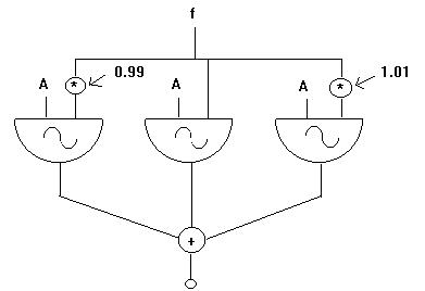
This diagram shows that the orchestra has three simultaneous oscillators, each one tuned slightly differently. The one in the middle is the unchanged frequency; the one on the left tunes down slightly by multiplying the input frequency by 0.99, and the one on the right tunes up slightly by multiplying the input frequency by 1.01.
The orchestra text file looks like this:
;chorus.orc
sr =   22050
kr =    1470
ksmps =   15
nchnls =   1

instr 4

inote = cpspch(p5)               ;convert octave.00 pitch notation to cps
k1  linen  10000,  p6,  p3,  p7  ;envelope shape each note
a1  oscil  k1,  inote * .99, 1	 ;pitch detuned down slightly
a2  oscil  k1,  inote * 1.01, 1  ;pitch detuned up slightly
a3  oscil  k1,  inote, 1         ;pitch unchanged
a1  = (a1+a2+a3)		 ;combine the 3 pitch variants
    out  a1
endin
In case of amplitude overload, the line which sums the outputs could be divided by 3: a1 = (a1+a2+a3)/3
In the octave.00 pitch notation, the 'octave' means which octave (middle C is octave 8); the '.00' notations are semitones between the octaves, from 0 (.00 = C) to 11 (.11 = B-natural).
This chart will help orientate you:
Csound pitch |
MIDI note |
Freq |
8.09 |
69 |
440 Hz |
3.00 |
0 |
8 Hz |
12.09 |
127 |
7040 Hz |
1.00 |
- |
2 Hz |
0.00 |
- |
1 Hz |
The sound is enriched by the combination of the original pitch with the versions detuned above and below. It is possible for the amplitude to get out of hand when combining pitches like this, so it would be wise to add something to the orchestra to handle this:
iamp  = ampdb(p4) ;get amp from p4 and convert decibel notation
to linear amplitude
iscale = iamp*.333 ;pre-divide (multiply *.333) each by a third so
that when added together they do not exceed the maximum value
The resulting changing amplitude value, 'iscale', is placed in the LINEN generator in place of a fixed amplitude value. Thus, instead of a single fixed amplitude value there is a changing set of values comprising the rise and fall of the envelope shape. Try to think about this for a moment and actually picture the whole envelope shape in place of the single value. Understanding how and where you can position whole shapes in place of single values is one of the keys to opening up the potential of Csound.
The i of 'iamp', 'iscale' and 'inote' means 'initialisation'. This means that Csound will do this operation at the beginning of each note of the score so that it will take on a single value. This is a good place to mention that Csound has three 'rates'. The other two are audio a and control k. In the audio rate, there is a value for every sample of sound. In the control rate, there is one value for a whole group of sound samples ksmps. A number of operations, such as envelopes, work perfectly well at this slower rate, and therefore save memory and processing time. Look back at the orchestras we've met so far and notice how some variables begin with the letter a (meaning 'audio rate') and others with k (meaning 'control rate').
When we create the score for this orchestra, there is another way that we can enrich the sound, and that is by enriching the partials of the sine wave generator. Up until now, we have only used the fundamental, thereby creating the purest of sine waves:
f1 0 4096 10 1
But GEN10 also allows us to set the harmonics, giving them an amplitude value relative to 1. So the next version of our score does this, giving the first harmonic a value of .1 and the second harmonic a value of .025. The first harmonic is an octave above the fundamental, and the second harmonic is a fifth above that (in line with the harmonic series):
f1 0 4096 1 .1 .025
One could take this process further, and also experiment with changing the weighting, making certain harmonics stronger and others weaker (in amplitude).
The score that follows plays a series of separate notes and then a series of chords. Note how the chorusing effect becomes richer with the chords.
;chorus2.sc

f1  0  4096  10  1  .1  .025  ;sine wave with 3 partials

;p1    p2    p3   p4    p5    p6     p7
;instr start dur  ampl  freq  attack release
i4     0     1    75    8.04  .1     .7
i4     1     1    70    8.02  .07    .6
i4     2     1    75    8.00  .05    .5
i4     3     1    70    8.02  .05    .4
i4     4     1    85    8.04  .1     .5
i4     5     1    80    8.04  .05    .5
i4     6     1    85    8.04  .03    .9
;chords begin here
i4     8     3    70    8.04  .03    .5
i4     8     3    72    8.00  .04    .5

i4     11    3    70    8.07  .03    .5
i4     11    3    72    8.04  .04    .5

i4     14    4    73    8.09  .03    .5
i4     14    4    72    8.05  .04    .5
i4     14    4    74    8.00  .05    .5

i4     18    4    73    8.07  .03    .5
i4     18.1  4    72    8.04  .04    .5
i4     18.2  4    74    8.00  .05    .5
e
Frequency Modulation ('FM') has proven to be a very effective method of enriching sound: it achieves remarkably complex results in a very simple way, though the predictability factor is not very high: small changes can result in dramatic, unexpected results.
Frequency modulation is a form of non-linear (ie irregular) audio distortion at higher frequencies and amplitudes. We are familiar with instrumental vibrato at low frequencies and amplitudes: a pitch wavers slightly up and down a few times a second. The perceived pitch is the relatively steady part of what we hear and is called, in this context, the 'carrier': because it 'carries' the slower, wavering component. The latter is called the 'modulator'.
First, a generic flow diagram for frequency modulation:
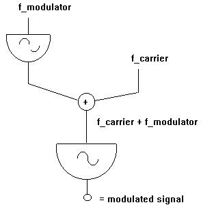
The orchestra for frequency modulation, really a simple vibrato instrument, is correspondingly straightforward:
;fm1.orc
sr  = 22050
kr   =  1470
ksmps = 15
nchnls =  1

instr 1
avib  oscil  p7, p6, 1		;p7 = modulation vibrato depth
		;p6 = modulation vibrato rate
aout  oscil  p4, p5 + avib, 1	;p4 = note amplitude ('carrier' volume)
		;p5 = note frequency ('carrier' pitch)
         out    aout
endin
If we revise what the components of the oscil generator are, we can see what's happening here. The three fields are amplitude, frequency and wavetable. We create the vibrato oscillation when we make 'avib', giving separate pfields in the score to hold the amplitude and frequency information. This is the modulator. We have to apply this to (combine this with) the carrier. This we do simply by adding it to the frequency field of the carrier. Thus the faster wave of the carrier has added to it the slower amplitude-frequency pattern of the modulator, and the modulator movement is heard to wobble the steadier carrier wave.
And now the score, using a simple sine wave, changing one parameter only in each group of notes:
;fm1.sc

f1 0 4096 10 1

;first, gradually increase the vibrato depth

;p1    p2    p3   p4     p5     p6       p7
;instr start dur  ampl   freq	vib.frq  vib.amp
i1      0    4    10000  440    5        0
i1      5    4    10000  440    5        3
i1     10    4    10000  440    5        6
i1     15    4    10000  440    5        10
i1     20    4    10000  440    5        15
;now hold vibrato depth steady and increase vibrato rate
i1     25    4    10000  440    2        4
i1     30    4    10000  440    5        4
i1     35    4    10000  440    7        4
i1     40    4    10000  440    12       4
i1     45    4    10000  440    20       4
i1     50    4    10000  440    100      4
;now we can seriously incease the modulation depth
i1     55    4    10000  440    100      10
i1     60    4    10000  440    100      50
i1     65    4    10000  440    100      100
i1     70    4    10000  440    100      500
i1     75    4    10000  440    100      1000
i1     80    4    10000  440    100      5000
;finally, we'll change the modulation frequency slightly
i1     85    4    10000  440    100      500
i1     90    4    10000  440    105      500
i1     95    4    10000  440    110      500
i1    100    4    10000  440    120      500
e
You must listen to this score – and think about the parameters – while you listen to the sound output.
It is clear, then, that we have with Csound complete and precise software control over the making of frequency modulation effects.
Yet another method by which we can enrich the sound is ring modulation. This was a familiar feature of many of the early analog synthesizers. It is achieved by a very simple process of multiplying together the output of two different oscillators; this distorts the harmonic ratios by creating sum & difference tones. (As waves can be expressed as sine functions, multiplying two waves means multiplying two sine functions. By the laws of trigonometry, this will involve the sum and difference of the two.)
This is expressed in a schematic way in the following flow diagram:
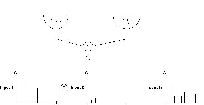
We can think about what happens by considering the graphs. When the two waves are multiplied together, a more complex pattern of partials emerges. The following orchestra and score illustrates ring modulation:
;rm1.orc - simple ring modulation instrument
sr  =    22050
kr  =     1470
ksmps =     15
nchnls =     1

;multiplication instrument

instr 1
a1  oscil  p6, p7, 1
a2  oscil  p4, p5, 1
      out    a1 * a2	;NB  * not +
endin

;simple oscillator for comparison
instr 2
a3  oscil  p4, p5, 1
      out    a3
endin
In the score below, note that the duration of the first event is 6 seconds; the second event comes in after three seconds, so they overlap, thus combining the sound of the two events; both are produced with the simple oscillator defined as instr 2. This is not ring modulation, but is here so that we can compare the two tones sounding together, i.e., added, and two tones multiplied together. After the initial 6 seconds, and we then hear the ring modulation effect for four seconds.
The s in the score is a section divider, used so that we can start each section at time 0.
The value given for amplitude2 in p6 is very low. The reason for this is that when a1 is multiplied by a2, the amplitudes are also multiplied (p6 * p4) resulting in the more normal value of 20000. We could have used equal amplitudes and then scaled the output as illustrated in the section on Chorusing.
;rm1.sc

f1 0 4096 10 1  ;sine wave

;p1    p2    p3   p4    p5    p6    p7
;instr start dur  amp   freq  amp2  freq2   ;comments
i2     0     6    2000  440                 ;tone 1
i2     3     3    2000  163                 ;tone 1+tone2
i1     6     4    2000  440   10    163     ;tone 1*tone2
s
i2     0     6    2000  440                 ;tone 1
i2     3     3    2000  420                 ;tone 1+tone2
i1     6     4    2000  440   10    420     ;tone 1*tone2
s
i2     0     6    2000  440                 ;tone 1
i2     3     3    2000  20                  ;tone 1+tone2
i1     6     4    2000  440   10    20      ;tone 1*tone2
s
i2     0     6    2000  440                 ;tone 1
i2     3     3    2000  881                 ;tone 1+tone2
i1     6     4    2000  440   10    881     ;tone 1*tone2
s
i2     0     6    2000  440                 ;tone 1
i2     3     3    2000  1000                ;tone 1+tone2
i1     6     4    2000  440   10    1000    ;tone 1*tone2
s
i2     0     6    2000  440                 ;tone 1
i2     3     3    2000  3864                ;tone 1+tone2
i1     6     4    2000  440   10    3864    ;tone 1*tone2
e
The Buzz unit generator automatically produces N partials – i.e., as many as you want: whatever value you enter for N. Thus you can produce quite a complex sound with one line of code. The example given here illustrates what happens as the number of partials is increased. The buzz orchestra is so amazingly simple that it's a very useful unit generator to explore, especially as the results are often rich enough to provide some good material.
;buzz1.orc - buzz orchestra

sr =   22050
kr =    1470
ksmps =   15
nchnls =   1

instr 1
k1  linen  p4, p6, p3, p7	;envelope
a1  buzz   k1, p5, p8, 1	;oscillator – p8 is N partials
      out    a1
endin
Buzz is therefore using a constant amplitude shape k1 as defined by linen (ampl-p4, attack-p6, duration-p3, decay-p7). The next parameter is pitch (p5) which in our score remains constant, then the number of partials (p8), which steadily increases in the score, and finally wavetable 1, again using only a simple sine wave.
In the score, note the use of dots as a way of repeating the parameter data. Also note that the frequency selected is very low. This brings more of the higher partials into a readily audible range, thus making the buzz effect more noticeable.
;buzz1.sc - buzz score

f1  0  8192  10  1	;note the larger table

;p1    p2    p3   p4    p5    p6    p7     p8
;instr start dur  ampl  freq  rise  decay  partials
i1     0     2    30000 40    .1    .1     5
i1     3     .    .     .      .     .     6
i1     6     .    .     .      .     .     7
i1     9     .    .     .      .     .     8
i1     12    .    .     .      .     .     10
i1     15    .    .     .      .     .     15
i1     18    .    .     .      .     .     20
i1     21    .    .     .      .     .     40
i1     24    .    .     .      .     .     80
e
It would be wonderful to go through all the unit generators of Csound in this way, but hopefully this will be sufficient to provide a good start on using this powerful tool. The next step could be to select another unit generator and explore it in a similar way. After that you could work through the Csound Tutorial by Richard Boulanger in the new Csound Reference Manual (now located here [R.F.]).
The Csound Book and The Csound Catalogue (ed. R. Boulanger) are also now available. These are absolute goldmines of information about all aspects of Csound.